Radius
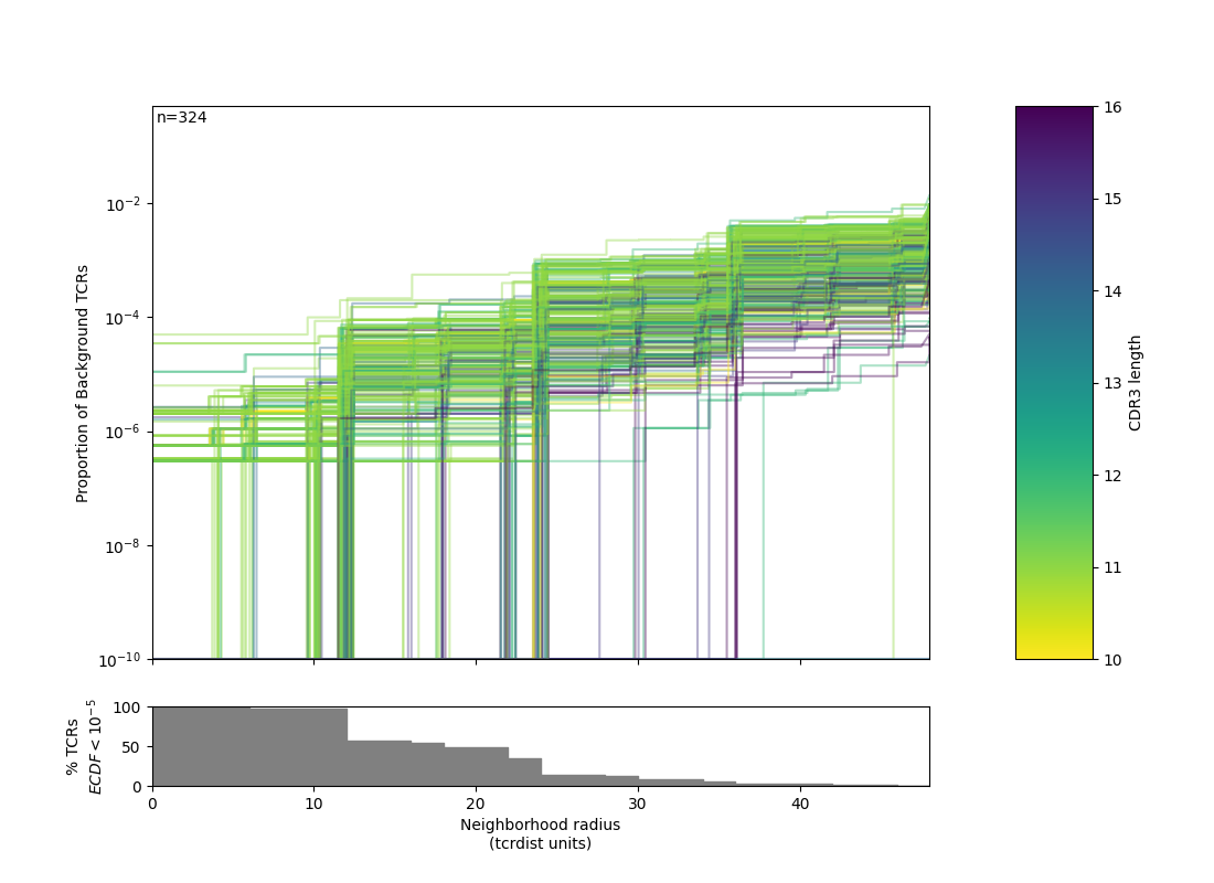
The utility of a TCR-based biomarker depends on antigen recognition. Therefore, a key constraint on distance-based clustering is the presence of similar TCR sequences that may lack the ability to recognize the target antigen. To be useful, a biochemical neighborhood definition should be wide enough to capture multiple biochemically similar TCRs with shared antigen-recognition, but not excessively broad as to include a high number of sequences found in background repertoires that are antigen-naive. Because the density of neighborhoods around TCRs are heterogeneous, we hypothesize that the optimal radius for grouping may differ according to properties of each TCR. To find an ideal radius we proposed comparing the relative density of a radius-defined target TCR neighborhood in the antigen-enriched repertoire to the density in a radius-defined neighborhood in an unenriched reference repertoire. Radii may be tuned based on how common a given query TCR is within an un-enriched bulk background repertoire. Due to biases in VDJ recombination, some TCRs will naturally have more neighbors. By contrast TCRs with rarer V-J pairings and more randomly inserted nucleotides will naturally have fewer neighbors, absent strong convergent selective pressure. tcrdist3 allows flexible discovery of TCR-specific search radii based on controlling an estimated rate of TCR-neighbor discovery in default or user-supplied control repertoires Inverse probability weighting may be used to more efficiently estimate background TCR discovery rate.
The following example shows how:
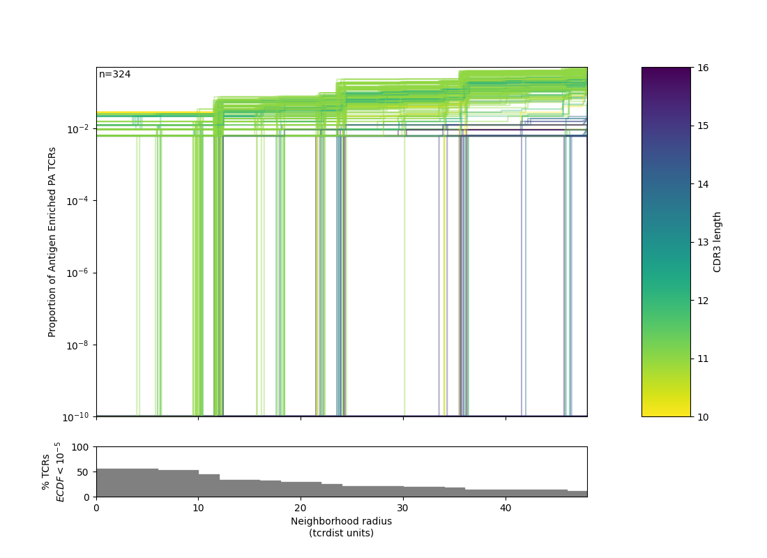
1 2 3 4 5 6 7 8 9 10 11 12 13 14 15 16 17 18 19 20 21 22 23 24 25 26 27 28 29 30 31 32 33 34 35 36 37 38 39 40 41 42 43 44 45 46 47 48 49 50 51 52 53 54 55 56 57 58 59 60 61 62 63 64 65 66 67 68 69 70 71 72 73 74 75 76 77 78 79 80 81 82 83 84 85 86 87 88 89 90 91 92 93 94 95 96 97 98 99 100 101 102 103 104 | """ Example of TCR radii defined for each TCR in an antigen enriched repertoire, and logo-motif report. """ import os import numpy as np import pandas as pd from tcrdist.repertoire import TCRrep from tcrdist.sample import _default_sampler from tcrdist.background import get_stratified_gene_usage_frequency from tcrdist.centers import calc_radii from tcrdist.public import _neighbors_sparse_variable_radius, _neighbors_variable_radius from tcrdist.public import TCRpublic from tcrdist.ecdf import _plot_manuscript_ecdfs import matplotlib.pyplot as plt # ANTIGEN ENRICHED REPERTOIRE # Load all TCRs tetramer-sorted for the epitope influenza PA epitope df = pd.read_csv("dash.csv").query('epitope == "PA"').\ reset_index(drop = True) # Load <df> into a TCRrep instance, to infer CDR1, CDR2, and CDR2.5 region of each clone tr = TCRrep(cell_df = df.copy(), organism = 'mouse', chains = ['beta'], db_file = 'alphabeta_gammadelta_db.tsv', compute_distances = True) # UN-ENRICHED REPERTOIRE # For illustration we pull a default sampler for mouse beta chains. # This is used to estimate the gene usage # probabilities P(TRBV = V, TRBJ = J) ts = _default_sampler(organism = "mouse", chain = "beta")() ts = get_stratified_gene_usage_frequency(ts = ts, replace = True) # Then we synthesize a background using Olga (Sethna et al. 2019), # using the P(TRBV = V, TRBJ = J) for inverse probability weighting. df_vj_background = tr.synthesize_vj_matched_background(ts = ts, chain = 'beta') # Load <df_vj_background> into a TCRrep instance, to infer CDR1,CDR2,CDR2.5 trb = TCRrep(cell_df = df_vj_background.copy(), organism = 'mouse', chains = ['beta'], db_file = 'alphabeta_gammadelta_db.tsv', compute_distances = False) # Take advantage of multiple CPUs tr.cpus = 4 # Compute radii for each TCR that controls neighbor-discovery in the background at # estimate of 1/10^5 inverse probability weighted TCRs. # Note we are set <use_sparse> to True, which allows us to take advantage of # multiple cpus and only store distance less than or equal to <max_radius> radii, thresholds, ecdfs = \ calc_radii(tr = tr, tr_bkgd = trb, chain = 'beta', ctrl_bkgd = 10**-5, use_sparse = True, max_radius=50) # Optional, set a maximum radius tr.clone_df['radius'] = radii tr.clone_df['radius'][tr.clone_df['radius'] > 26] = 26 # Tabulate index of neighboring clones in the ANTIGEN ENRICHED REPERTOIRE, # at each TCR-specific radius tr.clone_df['neighbors'] = _neighbors_variable_radius( pwmat = tr.pw_beta, radius_list = tr.clone_df['radius']) # Tabulate neighboring sequences in background tr.clone_df['background_neighbors'] = _neighbors_sparse_variable_radius( csrmat = tr.rw_beta, radius_list = tr.clone_df['radius']) # Tabulate number of unique subjects tr.clone_df['nsubject'] = tr.clone_df['neighbors'].\ apply(lambda x: tr.clone_df['subject'].iloc[x].nunique()) # Score Quasi(Publicity) : True (Quasi-Public), False (private) tr.clone_df['qpublic'] = tr.clone_df['nsubject'].\ apply(lambda x: x > 1) # OPTIONAL: HTML Report # Note: you can call TCRpublic() with fixed radius or directly # after tr.clone_df['radius'] is defined. tp = TCRpublic( tcrrep = tr, output_html_name = "quasi_public_clones.html") tp.fixed_radius = False # Generates the HTML report rp = tp.report() # OPTIONAL: ECDF Figure, against reference f1 = _plot_manuscript_ecdfs( thresholds = thresholds, ecdf_mat = ecdfs, ylab= 'Proportion of Background TCRs', cdr3_len=tr.clone_df.cdr3_b_aa.str.len(), min_freq=1E-10) f1.savefig(os.path.join("", "PA1.png")) from tcrdist.ecdf import distance_ecdf tresholds, antigen_enriched_ecdf = distance_ecdf( pwrect = tr.pw_beta, thresholds= thresholds, weights=None, pseudo_count=0, skip_diag=False, absolute_weight=True) # It is straightforward to make a ECDF between antigen enriched TCRs as well: antigen_enriched_ecdf[antigen_enriched_ecdf == antigen_enriched_ecdf.min()] = 1E-10 f2 = _plot_manuscript_ecdfs( thresholds = thresholds, ecdf_mat = antigen_enriched_ecdf, ylab= 'Proportion of Antigen Enriched PA TCRs', cdr3_len=tr.clone_df.cdr3_b_aa.str.len(), min_freq=1E-10) f2.savefig(os.path.join("", "PA2.png")) |
See PA QuasiPublic Meta Clonotypes.
Note: another conservative approach is to use a small fixed radius such as 16 TCRdist units (TDUs), this corresponds with 1-3 amino acid changes between CDR3s, depending on substituted residues.