Probability of Generation
Human Example
The generation probability, Pgen, defined by Walczyk and colleagues and implemented in Python by Sethna et al. (2019) is another way of filtering TCRs and TCR neighborhoods that are more frequent than expected based on their probability of being produced through recombination in early phases of immune development.
1 2 3 4 5 6 7 8 9 10 11 12 13 14 15 16 17 18 19 20 21 22 23 24 25 26 27 28 29 30 31 32 33 34 35 | """
How to add pgen estimates to human alpha/beta CDR3s
"""
import pandas as pd
from tcrdist.pgen import OlgaModel
from tcrdist import mappers
from tcrdist.repertoire import TCRrep
from tcrdist.setup_tests import download_and_extract_zip_file
df = pd.read_csv("dash_human.csv")
tr = TCRrep(cell_df = df.sample(5, random_state = 3),
organism = 'human',
chains = ['alpha','beta'],
db_file = 'alphabeta_gammadelta_db.tsv',
store_all_cdr = False)
olga_beta = OlgaModel(chain_folder = "human_T_beta", recomb_type="VDJ")
olga_alpha = OlgaModel(chain_folder = "human_T_alpha", recomb_type="VJ")
tr.clone_df['pgen_cdr3_b_aa'] = olga_beta.compute_aa_cdr3_pgens(
CDR3_seq = tr.clone_df.cdr3_b_aa)
tr.clone_df['pgen_cdr3_a_aa'] = olga_alpha.compute_aa_cdr3_pgens(
CDR3_seq = tr.clone_df.cdr3_a_aa)
tr.clone_df[['cdr3_b_aa', 'pgen_cdr3_b_aa', 'cdr3_a_aa','pgen_cdr3_a_aa']]
"""
cdr3_b_aa pgen_cdr3_b_aa cdr3_a_aa pgen_cdr3_a_aa
0 CASSETSGRSPYEQYF 1.922623e-09 CAVRPGYSSASKIIF 1.028741e-06
1 CASSPGLASPYSYNEQFF 1.554569e-11 CAVRVLMEYGNKLVF 1.128865e-08
2 CASSSRSTDTQYF 5.184760e-07 CAGAGGGSQGNLIF 2.512580e-06
3 CASSIGVYGYTF 8.576919e-08 CAFMSNAGGTSYGKLTF 1.832054e-07
4 CASSLLVSGVSSTDTQYF 2.143508e-11 CAVIGEGGKLTF 5.698448e-12
"""
|
If you want to compute many pgens this example shows how you can use parmap to accelerate the computation if you have multiple cores.
1 2 3 4 5 6 7 8 | """
Really simple example of using multiple cpus to
speed up computation of pgens with olga.
"""
import parmap
from tcrdist.pgen import OlgaModel
olga_beta = OlgaModel(chain_folder = "human_T_beta", recomb_type="VDJ")
parmap.map(olga_beta.compute_aa_cdr3_pgen, ['CASSYRVGTDTQYF', 'CATSTNRGGTPADTQYF', 'CASQGDSFNSPLHF', 'CASSPWTGSMALHF'])
|
Mouse Example
This example shows similar functionality for mouse data. It also illustrates how OLGA + tcrdist3 allow one to look for low probability of generation TCRs that have lots of biochemically similar neighbors, which can be a sign of strong convergent selection cause by antigen exposure.
1 2 3 4 5 6 7 8 9 10 11 12 13 14 15 16 17 18 19 20 21 22 23 24 25 26 27 28 29 30 31 32 33 34 35 36 37 38 39 40 41 42 43 44 45 46 47 48 49 50 51 52 53 54 55 56 57 58 59 60 61 62 63 64 65 66 67 68 69 70 71 72 73 74 75 76 77 78 79 80 81 82 83 84 85 86 87 88 89 90 91 92 93 94 95 96 97 98 99 100 101 102 103 104 105 106 107 108 109 110 111 112 113 114 115 116 117 118 119 120 121 122 123 124 125 126 127 128 129 130 131 132 | import pandas as pd
from tcrdist.repertoire import TCRrep
from tcrdist.pgen import OlgaModel
import numpy as np
df = pd.read_csv("dash.csv")
tr = TCRrep(cell_df = df,
organism = 'mouse',
chains = ['alpha','beta'],
db_file = 'alphabeta_gammadelta_db.tsv',
compute_distances = True)
# Load OLGA model as a python object
olga_beta = OlgaModel(chain_folder = "mouse_T_beta", recomb_type="VDJ")
olga_alpha = OlgaModel(chain_folder = "mouse_T_alpha", recomb_type="VJ")
# An example computing a single Pgen
olga_beta.compute_aa_cdr3_pgen(tr.clone_df['cdr3_b_aa'][0])
olga_alpha.compute_aa_cdr3_pgen(tr.clone_df['cdr3_a_aa'][0])
# An example computing multiple Pgens
olga_beta.compute_aa_cdr3_pgens(tr.clone_df['cdr3_b_aa'][0:5])
olga_alpha.compute_aa_cdr3_pgens(tr.clone_df['cdr3_a_aa'][0:5])
# An example computing 1920 Pgens more quickly with multiple cpus
import parmap
tr.clone_df['pgen_cdr3_b_aa'] = \
parmap.map(
olga_beta.compute_aa_cdr3_pgen,
tr.clone_df['cdr3_b_aa'],
pm_pbar=True,
pm_processes = 2)
tr.clone_df['pgen_cdr3_a_aa'] = \
parmap.map(
olga_alpha.compute_aa_cdr3_pgen,
tr.clone_df['cdr3_a_aa'],
pm_pbar=True,
pm_processes = 2)
"""
We can do something else useful. We've tweaked the original
generative code in OLGA, so that you can generate CDRs,
given a specific TRV and TRJ.
Note that unfortunately not all genes are recognized in default OLGA models,
but many are. This gives you an idea of what you can do. Here are 10
CDR3s generated at random given a particular V,J usage combination
"""
np.random.seed(1)
olga_beta.gen_cdr3s(V = 'TRBV14*01', J = 'TRBJ2-5*01', n =10)
olga_alpha.gen_cdr3s(V ='TRAV4-3*02', J ='TRAJ31*01', n =10)
"""
Using this approach, we can synthesize an 100K background,
with similar gene usage frequency to our actual repertoire.
Note, however, that given data availability,
this is currently likely the most reliable for human beta chain.
After OLGA's publication, a default mouse alpha model (mouse_T_alpha)
was added to the OLGA GitHub repository. We've included that here
but it should be used with caution as it is missing
a number of commonly seen V genes.
"""
np.random.seed(1)
tr.synthesize_vj_matched_background(chain = 'beta')
"""
v_b_gene j_b_gene cdr3_b_aa pV pJ pVJ weights source
0 TRBV14*01 TRBJ2-3*01 CASSLASAETLYF 0.033721 0.092039 0.002989 0.065742 vj_matched
1 TRBV13-2*01 TRBJ2-3*01 CASGDAPDRTGAETLYF 0.118785 0.092039 0.010331 0.271309 vj_matched
2 TRBV13-3*01 TRBJ1-1*01 CASSDGFSRTGGVNTEVFF 0.074051 0.106146 0.006923 1.009124 vj_matched
3 TRBV13-3*01 TRBJ2-1*01 CASSDVQGGAEQFF 0.074051 0.117684 0.008915 1.021244 vj_matched
4 TRBV13-3*01 TRBJ2-7*01 CASSSGTGGYIYEQYF 0.074051 0.204898 0.015366 1.670224 vj_matched
... ... ... ... ... ... ... ... ...
99995 TRBV14*01 TRBJ2-3*01 CASSPTGGAPYASAETLYF 0.033721 0.092039 0.002989 0.065742 vj_matched
99996 TRBV17*01 TRBJ2-5*01 CASSRDPTQDTQYF 0.028110 0.124712 0.004930 0.650360 vj_matched
99997 TRBV14*01 TRBJ2-3*01 CASSSTGGAETLYF 0.033721 0.092039 0.002989 0.065742 vj_matched
99998 TRBV13-1*01 TRBJ2-1*01 CASSDWGKDYAEQFF 0.106042 0.117684 0.013373 2.622194 vj_matched
99999 TRBV4*01 TRBJ2-3*01 CASSYDRGSAETLYF 0.040749 0.092039 0.002989 0.068343 vj_matched
"""
np.random.seed(1)
tr.synthesize_vj_matched_background(chain = 'alpha')
"""
v_a_gene j_a_gene cdr3_a_aa pV pJ pVJ weights source
0 TRAV12N-3*01 TRAJ34*02 CAIASNTNKVVF 0.000438 0.000088 0.000088 0.006059 vj_matched
1 TRAV3D-3*02 TRAJ33*01 CAVSAGADSNYQLIW 0.000088 0.000088 0.000088 0.005122 vj_matched
2 TRAV3-3*01 TRAJ27*01 CAVSTNTGKLTF 0.014029 0.042964 0.000877 0.277471 vj_matched
3 TRAV3-3*01 TRAJ26*01 CAVSHNYAQGLTF 0.014029 0.040947 0.001052 0.009155 vj_matched
4 TRAV3-3*01 TRAJ26*01 CAVSARNYAQGLTF 0.014029 0.040947 0.001052 0.009155 vj_matched
... ... ... ... ... ... ... ... ...
99995 TRAV3D-3*02 TRAJ21*01 CAVSVSNYNVLYF 0.000088 0.039982 0.000088 0.003758 vj_matched
99996 TRAV3-3*01 TRAJ43*01 CAVSENNNNAPRF 0.014029 0.022271 0.000526 0.071093 vj_matched
99997 TRAV3D-3*02 TRAJ26*01 CAVSGNYAQGLTF 0.000088 0.040947 0.000088 0.000296 vj_matched
99998 TRAV3-3*01 TRAJ26*01 CAVKGNNYAQGLTF 0.014029 0.040947 0.001052 0.009155 vj_matched
99999 TRAV9N-2*01 TRAJ15*01 CTYQGGRALIF 0.000088 0.043840 0.000088 0.020438 vj_matched
"""
""""
tcrdist3's integration of Pgen estimates makes it very easy to look for
PUBLIC clusters of TCRs (i.e. high number of neighbors) with unlikely V(D)J
recombinations.
"""
from tcrdist.public import _neighbors_fixed_radius
from tcrdist.public import _K_neighbors_fixed_radius
tr.clone_df['neighbors'] = _neighbors_fixed_radius(pwmat = tr.pw_beta, radius = 18)
tr.clone_df['K_neighbors'] = _K_neighbors_fixed_radius(pwmat = tr.pw_beta , radius = 18)
tr.clone_df['pgen_cdr3_b_aa_nlog10'] = tr.clone_df['pgen_cdr3_b_aa'].apply(lambda x : -1*np.log10(x))
tr.clone_df['nsubject'] = tr.clone_df['neighbors'].apply(lambda x: len(tr.clone_df['subject'][x].unique()))
# nsubject > 1 implies quasi-publicity
tr.clone_df['qpublic'] = tr.clone_df['nsubject'].apply(lambda x: x >1)
# Note one can find neighbors based on paired-chain distances.
from tcrdist.public import _neighbors_fixed_radius
from tcrdist.public import _K_neighbors_fixed_radius
tr.clone_df['neighbors'] = _neighbors_fixed_radius(pwmat = tr.pw_beta + tr.pw_alpha, radius = 50)
tr.clone_df['K_neighbors'] = _K_neighbors_fixed_radius(pwmat = tr.pw_beta + tr.pw_alpha , radius = 50)
tr.clone_df['pgen_cdr3_b_aa_nlog10'] = tr.clone_df['pgen_cdr3_b_aa'].apply(lambda x : -1*np.log10(x))
tr.clone_df['nsubject'] = tr.clone_df['neighbors'].apply(lambda x: len(tr.clone_df['subject'][x].unique()))
# nsubject > 1 implies quasi-publicity)
tr.clone_df['qpublic'] = tr.clone_df['nsubject'].apply(lambda x: x >1 )
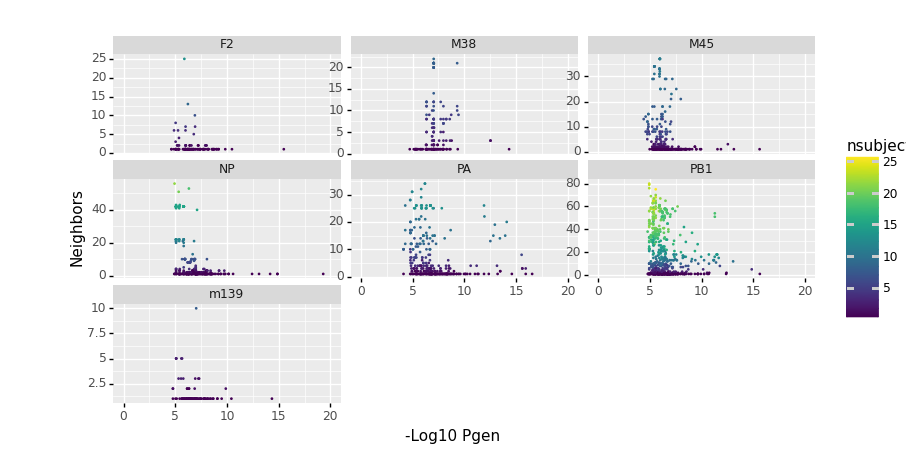
"""
#Code for plotting pgen vs. neighbors
import plotnine
from plotnine import ggplot, geom_point, aes, ylab, xlab
(ggplot(tr.clone_df,
aes(x= 'pgen_cdr3_b_aa_nlog10',
y ='K_neighbors',
color = 'nsubject')) +
geom_point(size = .1) +
plotnine.scales.xlim(0,20) +
plotnine.facets.facet_wrap('epitope', scales = "free_y")+ ylab('Neighbors') + xlab('-Log10 Pgen'))
"""
|
References
Zachary Sethna, Yuval Elhanati, Curtis G Callan, Aleksandra M Walczak, Thierry Mora Bioinformatics (2019) OLGA: fast computation of generation probabilities of B- and T-cell receptor amino acid sequences and motifs